Identify and measure key metrics to analyze the company performance

1. Introduction

To help readers gain a deeper understanding of the topic's context, I will use a use case from a real company with data published available on Kaggle. (Brazilian E-Commerce Public Dataset by Olist)

Olist – the Brazilian marketplace connects small businesses from all over Brazil to channels without hassle and with a single contract. Those merchants can sell their products through the Olist Store and ship them directly to the customers using Olist logistics partners.

They public a dataset about information on 100k orders from 2016 to 2018 made at multiple marketplaces in Brazil. Its features allow viewing an order from multiple dimensions: from order status, price, payment, and freight performance to customer location, product attributes, and finally reviews written by customers.

The big question is: What can we do with this dataset? How can we use it to evaluate company performance and deliver insights for improvement?

I'll outline some straightforward steps to answer two questions above

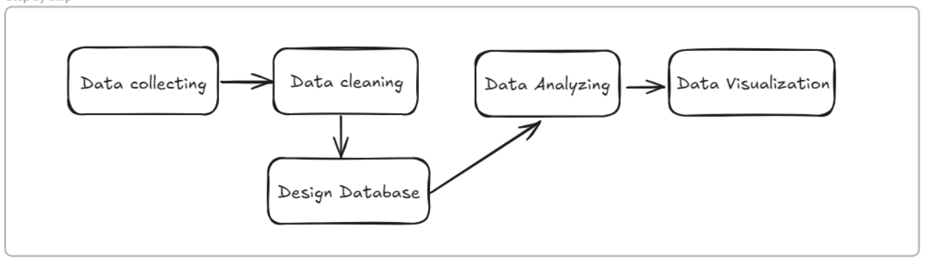
2. Tools support

Python (3.11)
SQL server
Power BI desktop

3. Data collecting

Collecting or prepare data help you read, understand data and store it for further analysis. Data Olist published is SQL database, so collected data can be stored in some SQL database like: Oracle (SQL Developer), MS SQL (Microsoft SQL),....

Here is their dataset: Brazilian E-Commerce Public Dataset by Olist (kaggle.com)

olist_customers_dataset.csv
olist_geolocation_dataset.csv
olist_order_items_dataset.csv
olist_order_payments_dataset.csv
olist_order_reviews_dataset.csv
olist_orders_dataset.csv
olist_products_dataset.csv
olist_sellers_dataset.csv
product_category_name_translation.csv

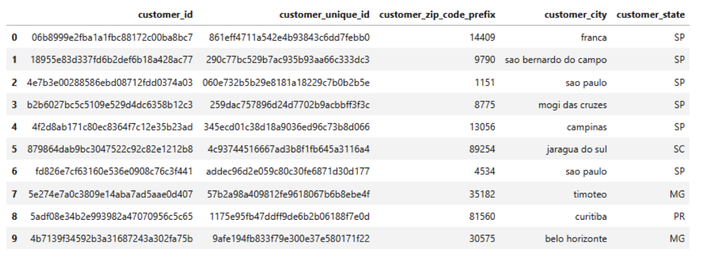
Read data by Python using familiar lib "pandas" :

1import pandas as pd
2customers = pd.read_csv("C:/Users/Admin/Documents/Dataset/olist_customers_dataset.csv")
3customers.head(10)

4. Design Database

When receiving a dataset, understanding the relationships between tables and defining dim-fact table is essential. It is useful for understanding the data context, enabling data analysis and decision-making, ensuring data accuracy and integrity, and enhancing performance and scalability.

4.1 First step

To design Database, we need to define which table is dimension table, which table is fact table. During the defining process, you will also gain a clear understanding of the data context and how to use it.

Dimension tables are tables that stores descriptive attributes.
- Think of dimension tables as the “who, what, where, and when” of your data. They contain descriptive information about the main subjects of your analysis.
- Dimension tables usually contains unique value (Each row represents a unique value and its details.) => Based on tables description and sample value, we can define that tables are dimension tables:

Table Name	Description	Primary Key
olist_customers_dataset	Contains information about customers and their locations.	#customer_unique_id
olist_geolocation_dataset	Contains Brazilian zip codes and their latitude/longitude coordinates.	#geolocation_zip_code_prefix
olist_orders_dataset	Contains information about all orders and their statuses.	#order_id
olist_products_dataset	Includes data about the products sold by Olist.	#product_id
olist_sellers_dataset	Includes data about the sellers fulfilling orders made at Olist.	#seller_id
product_category_name_translation	Includes product category names in Portuguese and their translations.	#product_category_name

Fact tables are tables that restores quantitative data (facts) related to events, activities, transactions,....
- Think of the fact table as the “how much”. It contains measurable data that represents the performance of a business process.
- A fact table contains key values from the dimension tables, but in different events or contexts, so the key values will be repeated based on those events or contexts. => Similarly, we can easily identify the fact tables:

Table Name	Description	Foreign Key
olist_order_items_dataset	Includes data about the items (products) purchased within each order, showing seller details.	#order_id, #product_id, #seller_id
olist_order_payments_dataset	Includes data about the payment options for orders. Each order_id may have multiple payment methods.	#order_id
olist_order_reviews_dataset	Includes data about customer reviews. One order_id can have multiple reviews on different dates.	#order_id

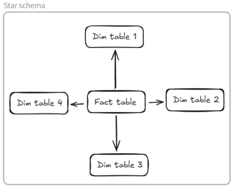
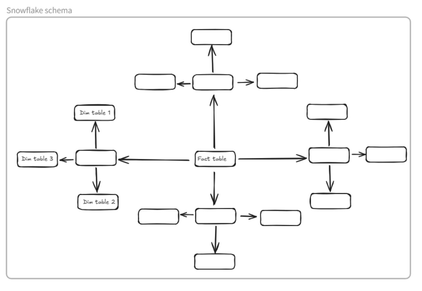
4.2 Next step: define type of schema.

Typically, for tables with a single fact table connected to multiple dimension tables via a single relationship link, a star schema (the simplest schema) is used. However, in this database, a dimension table can act as a fact table for another dimension table, so we need to use a snowflake schema.

4.3 Final step:

Connect the tables together using the Primary keys and Foreign keys identified above. Below is simple designed database built on MS SQL server:

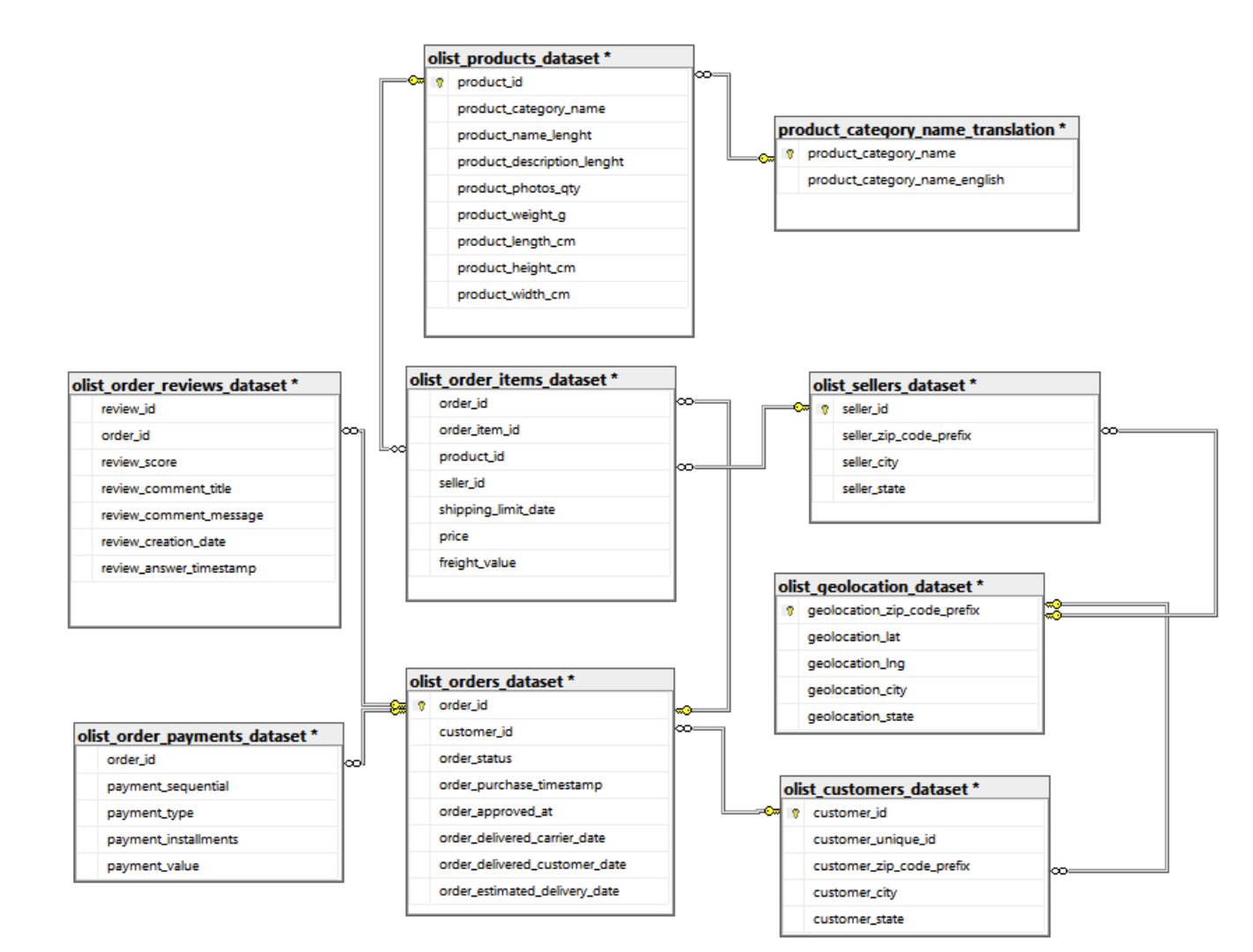
By looking at the designed database, it's easy to identify which tables are linked through which primary and foreign keys. This makes the process of calculating and using the data for analysis more transparent and helps to quickly understand the business context.

5. Data cleaning

Data during the entry and collection process from multiple sources can lead to misspellings, redundancies, and irrelevance. Clean data largely depends on data integrity. There might be duplicate data or the data might not be in a format, therefore the unnecessary data is removed and cleaned.

The two simplest metrics commonly used to check data quality are: checking for duplicate values and checking for null values.

Function for check all tables with 2 metrics:

1def overview_data(table_name):
2    nrows=table_name.shape[0]
3    ncols=table_name.shape[1]
4    null_values = table_name.isnull().sum()    
5    name_nul_cols = []
6    dups = [table_name.duplicated().sum()]
7    for i in range(len(null_values)):
8        if null_values[i] >0:
9            name_nul_cols.append(null_values.index[i])    
10    num_nul_cols = len(name_nul_cols)
11    return nrows, ncols , name_nul_cols,num_nul_cols, dups

1detailed_db = pd.DataFrame()
2list_dataset= [customers,geolocation,order_items,order_payments,order_reviews,orders,products,sellers]
3list_dataset_name= ['customers','geolocation','order_items','order_payments','order_reviews','orders','products','sellers']
4detailed_db['table_name'] = [i for i in list_dataset_name]
5detailed_db['no_rows'] = [overview_data(i)[0] for i in list_dataset]
6detailed_db['n_cols'] = [overview_data(i)[1] for i in list_dataset]
7detailed_db['names_of_null_cols'] = [', '.join(overview_data(i)[2]) for i in list_dataset]
8detailed_db['num_null_cols'] = [overview_data(i)[3] for i in list_dataset]
9detailed_db['num_dups'] = [overview_data(i)[4] for i in list_dataset]
10detailed_db

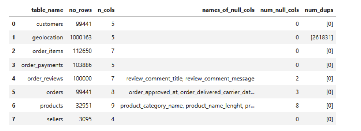
a. Duplicate values

As you see, table geolocation have many duplicate values, though this table is a dim table (primary key is geolocation_zip_code_prefix).

1geolocation.duplicated().sum()
2###279667

1### remove duplicate
2geolocation.drop_duplicates(inplace=True)

b. Null values

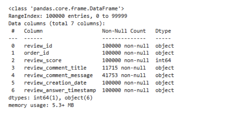
Order reviews tables: The two columns with null values in the table are not too important, and not every order will have a customer review, as this is an optional information field, so I will skip over these cases.

1order_reviews.info()

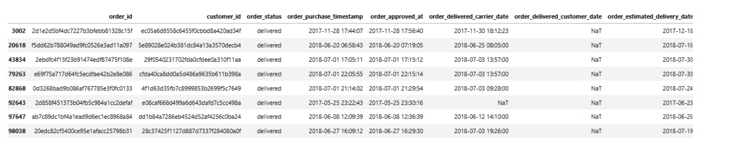
Order tables have null values but most of them are in non-delivered status (so null deliver_times are sensible).

1orders.loc[orders['order_delivered_customer_date'].isnull(), 'order_status'].unique()

There are 8 null values in delivered status but we can skip because of tiny values.

1orders.loc[orders['order_delivered_customer_date'].isnull() & (orders['order_status'] == 'delivered')]

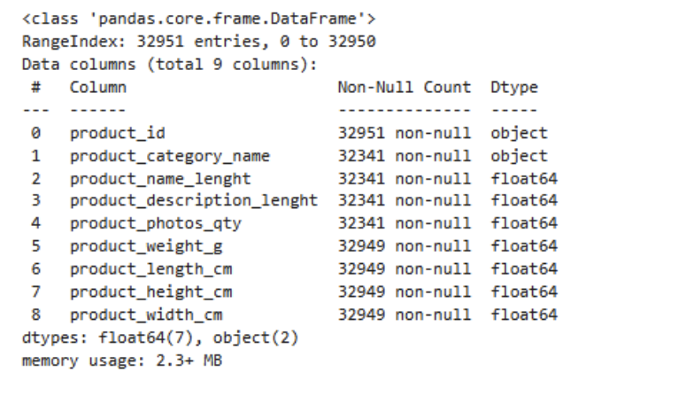
The products table shows that most columns have a low percentage of missing values (null_value < 2%). This suggests that the data is mostly complete.

1products.info()

c. Wrong data format

- Non-encode values

1geolocation['geolocation_city'].unique()

1### handle non-encode value
2geolocation['geolocation_city'] =  geolocation['geolocation_city'].apply(lambda x: unidecode(x) if isinstance(x, str) else x)
3geolocation['geolocation_city'].unique()

- Wrong pattern value

1special_delimiters = r'[,:\*\.;]'
2geolocation[geolocation['geolocation_city'].str.contains(special_delimiters)]

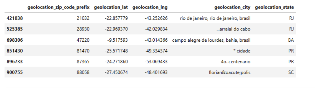
1### manual fix
2replacements = {
3    'rio de janeiro, rio de janeiro, brasil': 'rio de janeiro',
4    '...arraial do cabo': 'arraial do cabo',
5    'campo alegre de lourdes, bahia, brasil' : 'campo alegre de lourdes',
6    '* cidade' : 'cidade gaucha',
7    '4o. centenario' : '4o centenario',
8    'florian&oacute;polis' : 'florianopolis'
9}
10
11geolocation['geolocation_city'] = geolocation['geolocation_city'].replace(replacements)

- There are many latitude and longitude values for the same zip code

1check_dup_zip_code = geolocation[geolocation['geolocation_zip_code_prefix'] > 1].sort_values(by='geolocation_zip_code_prefix')
2check_dup_zip_code

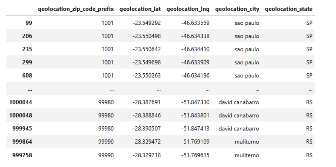
Since the latitude and longitude values are quite similar to each other, I will resolve this by taking the average of the values.

1geolocation_lat_mean = geolocation.groupby('geolocation_zip_code_prefix')['geolocation_lat'].transform('mean')
2geolocation_lng_mean = geolocation.groupby('geolocation_zip_code_prefix')['geolocation_lng'].transform('mean')
3
4# Update it into mean value
5geolocation['geolocation_lat'] = geolocation_lat_mean
6geolocation['geolocation_lng'] = geolocation_lng_mean

6. Data visualization and analyzing

Dashboard

I proposed a dashboard built by Power BI.

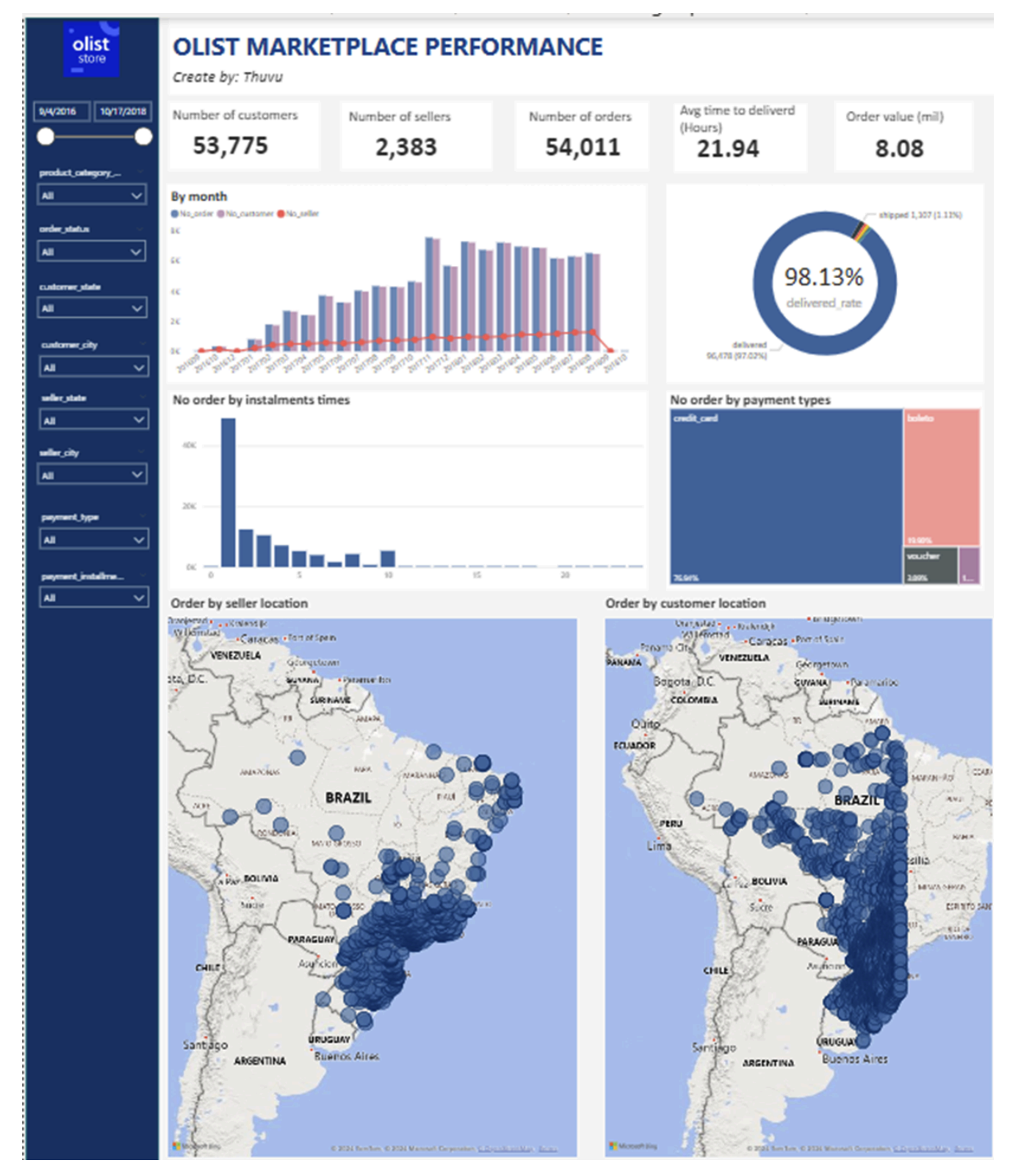
=> Some initial observations:

The number of orders is not significantly higher than the number of customers, indicating that most customers only made an order over the nearly 3-year period. This suggests that customers are not making frequent purchases, which could lead to customer churn.
There is a significant spike in the number of orders starting from November 2017, where the number of orders nearly doubled and then maintained that elevated level until the end of the reporting period. This suggests that Olist underwent some changes around this time, which could provide valuable lessons for the business.
The majority of the orders were delivered.
Since customers tend to use credit card as payment method, so the proportion of customers choosing installments are usually not very high.
The number of customers is heavily concentrated in the central regions, while the sellers are more concentrated in the western regions. This geographical mismatch could lead to higher shipping costs for Olist compared to other marketplaces.

Supporting analyst

By product

- Overview top 10 and bottom 10 product

1# Group by product_id and sum the total_value
2product_totals = df.groupby('product_category_name_english')['total_value'].sum().reset_index()
3
4# Sort the DataFrame by total_value in descending order and get the top 10 products
5top_10_products = product_totals.sort_values('total_value', ascending=False).head(10)
6
7bottom_10_products = product_totals.sort_values('total_value', ascending=False).tail(10)
8
9# Create the top 10 products chart
10top_10_fig = go.Figure(data=[go.Bar(
11    x=top_10_products['product_category_name_english'],
12    y=top_10_products['total_value']
13)])
14top_10_fig.update_layout(
15    title='Top 10 Products by Total Value',
16    xaxis_title='Product ID',
17    yaxis_title='Total Value'
18)
19
20# Create the bottom 10 products chart
21bottom_10_fig = go.Figure(data=[go.Bar(
22    x=bottom_10_products['product_category_name_english'],
23    y=bottom_10_products['total_value']
24)])
25bottom_10_fig.update_layout(
26    title='Bottom 10 Products by Total Value',
27    xaxis_title='Product ID',
28    yaxis_title='Total Value'
29)
30
31# Display the charts
32top_10_fig.show()
33bottom_10_fig.show()

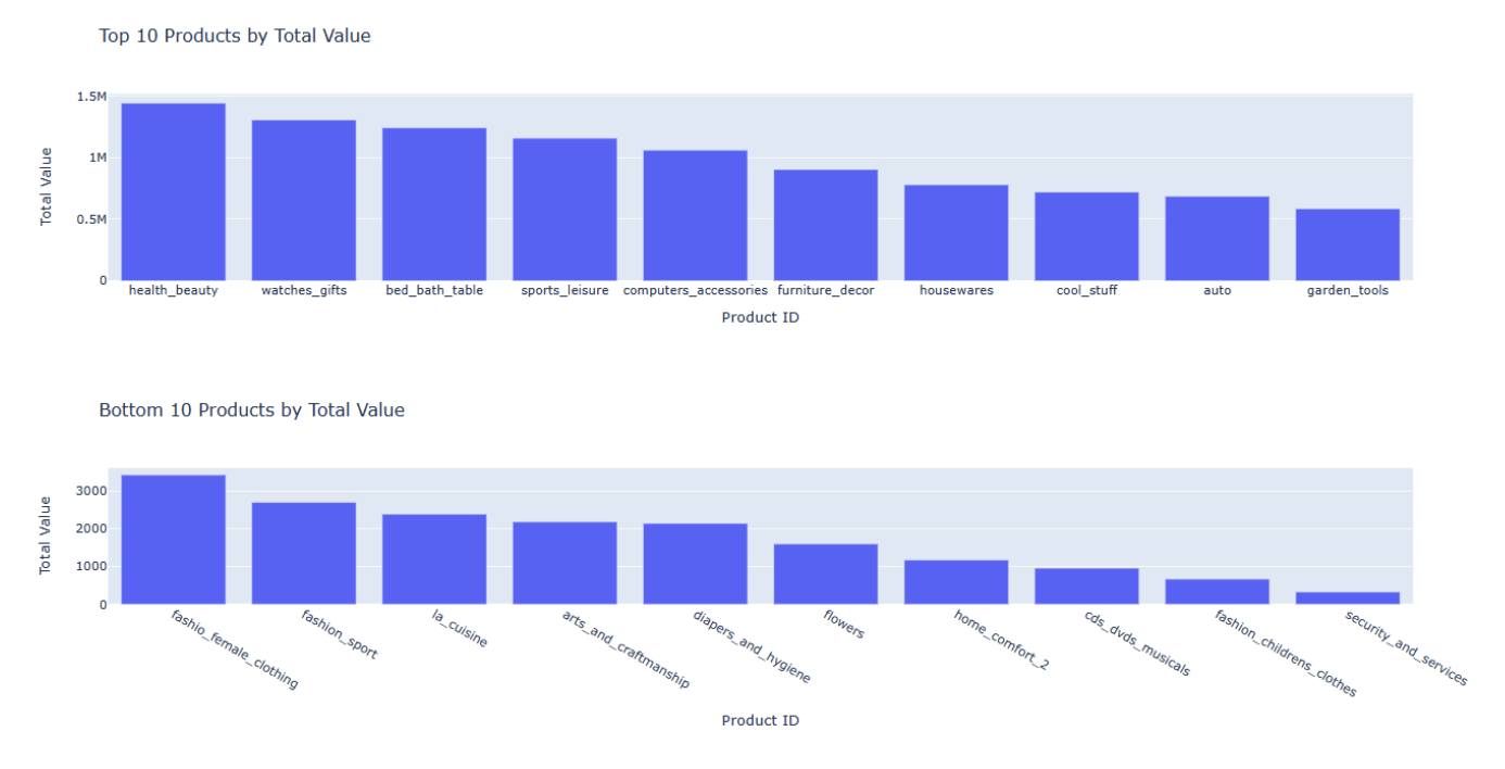
Based on the top 10 most ordered products, it appears that Olist's customers are primarily interested in furniture, home goods, and household items. As for the bottom 10 products, it appears that Olist's customers are less interested in products related to arts, sports, or services. This could be due to the lack of product diversity among Olist's sellers or the pricing may not be competitive enough in these categories.

- Relationship between product and other features

1df_boxplot = df[['product_name_lenght','product_description_lenght','product_photos_qty','product_weight_g','product_length_cm','product_height_cm','product_width_cm']]
2fig, axes = plt.subplots(nrows=2, ncols=4, figsize=(16, 8))
3
4for i, ax in enumerate(axes.flat):
5    if i < len(df_boxplot.columns):
6        df_boxplot[df_boxplot.columns[i]].plot(kind='box', ax=ax)
7        ax.set_title(df_boxplot.columns[i])
8    
9plt.suptitle('Boxplots of product features')
10plt.tight_layout()
11plt.show()

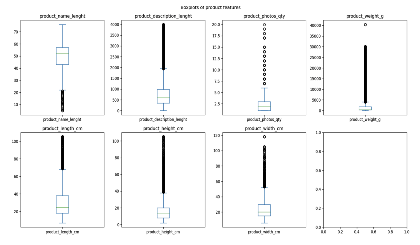
For products with longer names or descriptions, there tend to be more purchases by customers. However, the number of photos for a product does not seem to significantly influence the volume of customer purchases.

Olist's customers appear to prefer purchasing lightweight and compact products. This could suggest that they may not fully trust Olist's delivery capabilities or that the shipping costs for larger items are higher, deterring customers from making such purchases.

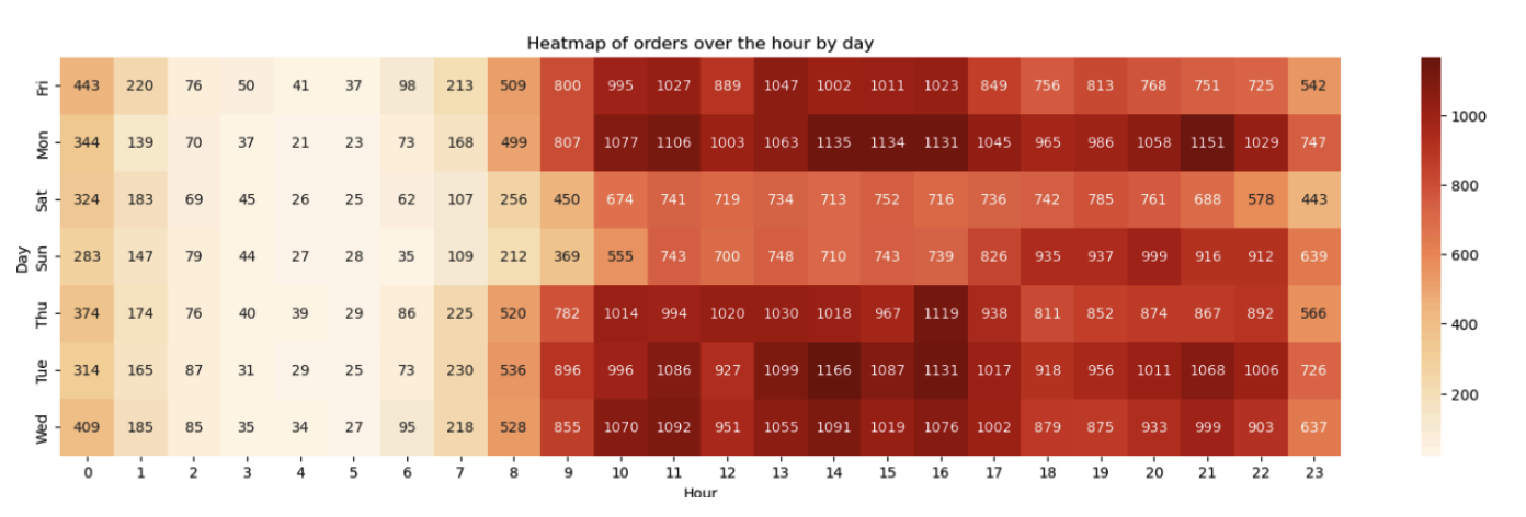
Orders over hour by day

Based on the chart, it can be seen that customers tend to make more purchases on weekdays rather than weekends. The traffic also appears to be higher during midday and afternoon hours compared to other times.

1plt.figure(figsize=(20, 5))
2day_hour=day_hour.pivot(index = 'weekday', columns = 'hour', values = 'freq')
3ax=sns.heatmap(day_hour, annot = True, fmt = "d", cmap = "OrRd")
4ax.set_xlabel("Hour")
5ax.set_ylabel("Day")
6ax.set_title("Heatmap of orders over the hour by day")

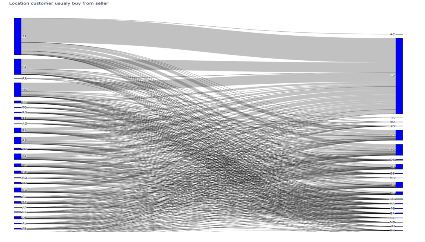
Order location distribution

From the chart, we can see that the majority of sellers are from the SP state (almost 50% of all), while there is also a significant number of buyers from the RJ state. However, these RJ buyers are mainly purchasing from the SP sellers. This geographical mismatch between buyers and sellers could result in very high shipping costs due to the inter-state nature of the transactions.

1sankey_data = df.groupby(['customer_state', 'seller_state'])['freight_value'].sum().reset_index()
2
3# Get the unique values for customer_state and seller_state
4customer_states = sankey_data['customer_state'].unique()
5seller_states = sankey_data['seller_state'].unique()
6
7# Create the Sankey diagram
8fig = go.Figure(data=[go.Sankey(
9    node=dict(
10        pad=15,
11        thickness=20,
12        line=dict(color="black", width=0.5),
13        label=list(customer_states) + list(seller_states),
14        color="blue"
15    ),
16    link=dict(
17        source=[list(customer_states).index(x) for x in sankey_data['customer_state']],
18        target=[len(customer_states) + list(seller_states).index(y) for y in sankey_data['seller_state']],
19        value=sankey_data['freight_value'],
20        label=[f"From {sankey_data['customer_state'][i]} to {sankey_data['seller_state'][i]}" for i in range(len(sankey_data))]
21    )
22)])
23
24fig.update_layout(title_text="Location customer usualy buy from seller", font_size=10,width=1300,  # Set the width of the chart
25    height=1000)
26fig.show()

7. Conclusion

Business decision-making:

1. Target new customer: To expand brand recognition and reach the entire Brazilian customer base, Olist should consider running broader marketing campaigns and initiatives. This could help increase their visibility and appeal to customers beyond the current geographical concentration.

2. Existing customer retention:

Utilize algorithms to provide personalized product recommendations based on their previous purchasing behavior and preferences.
Offer loyalty rewards or appreciation vouchers to incentivize repeat business from these valued customers.

3. Optimize the location-based structure Provide recommendations to sellers to locate their businesses closer to the high-demand customer clusters. This can help minimize shipping costs and delivery times.

4. Optimize the location-based structure Provide recommendations to sellers to locate their businesses closer to the high-demand customer clusters. This can help minimize shipping costs and delivery times.

Identify and Measure Key Metrics to Analyze the Company’s Performance

Table of Contents