Continuous Model Monitoring in Machine Learning (Part 2): Performance, Automation, and Action
Welcome back! In Part 1, we laid the foundation for robust ML model monitoring, exploring why it's essential, understanding drift, and detailing how to monitor your model's input features using techniques like null checks, percentile tracking, and Population Stability Index (PSI). Now that we understand how to keep an eye on the data going into the model, Part 2 focuses on what comes out and how to manage the monitoring process effectively. We'll dive into monitoring model predictions and actual performance, automating these checks with Apache Airflow, visualizing the results for clear insights, and establishing strategies for responding when drift inevitably occurs. Here's what we'll cover in Part 2: 5. Model Performance & Output Monitoring (Prediction PSI, Metrics like AUC/F1, Calibration) 6. Automating Monitoring with Apache Airflow 7. Visualizing Insights for Action 8. Responding to Drift: Strategies for Resilience 9. Best Practices and Next Steps 10. Conclusion 11. References
5. Model Performance & Output Monitoring
Beyond input features, we must monitor the model's outputs and, when possible, its actual performance against ground truth.
Monitoring Prediction Distributions (using PSI)
Even without ground truth labels, monitoring the distribution of your model's prediction scores using PSI is crucial. A significant shift (high PSI) often indicates that the model is reacting differently to the incoming data, possibly due to data drift or concept drift.
1import pandas as pd
2import numpy as np
3import logging
4# Simulate realistic data (e.g., fraud detection scores)
5np.random.seed(42)
6ref_data = pd.DataFrame({
7        'score': np.clip(np.random.normal(0.5, 0.1, 1000), 0.01, 0.99),
8    'label': (np.random.normal(0, 0.2, 1000) + 0.5 > 0.6).astype(int)
9})
10new_data = pd.DataFrame({
11        'score': np.clip(np.random.normal(0.6, 0.15, 1000), 0.01, 0.99),
12    'label': (np.random.normal(0, 0.25, 1000) + 0.6 > 0.65).astype(int)
13})
14def calculate_psi(ref_series: pd.Series, new_series: pd.Series, bins: int = 10) -> float:
15    """Calculate PSI between two distributions with proper edge case handling."""
16    if not pd.api.types.is_numeric_dtype(ref_series) or not pd.api.types.is_numeric_dtype(new_series):
17        logging.error("Non-numeric data provided for PSI calculation.")
18        return np.nan
19    ref_clean = ref_series.dropna()
20    new_clean = new_series.dropna()
21    if ref_clean.empty or new_clean.empty:
22        logging.warning("Empty data after dropping NaNs—PSI undefined.")
23        return np.inf
24    try:
25        # Use consistent bin edges based on combined range
26        min_val = min(ref_clean.min(), new_clean.min())
27        max_val = max(ref_clean.max(), new_clean.max())
28        bins_edges = np.linspace(min_val, max_val, bins + 1)
29        ref_hist, _ = np.histogram(ref_clean, bins=bins_edges, density=True)
30        new_hist, _ = np.histogram(new_clean, bins=bins_edges, density=True)
31        ref_hist += 1e-10  # Avoid log(0)
32        new_hist += 1e-10
33        psi = np.sum((new_hist - ref_hist) * np.log(new_hist / ref_hist))
34        return float(psi)
35    except Exception as e:
36        logging.error(f"Error calculating PSI: {e}")
37        return np.nan
38psi_score = calculate_psi(ref_data['score'], new_data['score'])
39logging.basicConfig(level=logging.INFO)
40if psi_score > 0.2:
41    logging.warning(f"Significant drift in predictions: PSI={psi_score:.3f}")
42else:
43    logging.info(f"Prediction distribution stable: PSI={psi_score:.3f}")
Why It Matters:
- A stable score distribution suggests the model perceives the incoming data similarly to the training data. A drifting score distribution is a strong early warning sign that model performance might be degrading, even before labeled data confirms it.
- A high PSI (>0.2) hints at data or concept drift, prompting investigation before performance tanks.
Monitoring Performance Metrics (Requires Ground Truth)
When ground truth labels become available (even with a delay), you can directly measure model performance using standard metrics like AUC-ROC, F1-Score, Precision, Recall, Accuracy, LogLoss, etc., depending on your model type and business objective. Tracking these metrics over time is the ultimate validation of model health.
1from sklearn.metrics import roc_auc_score, f1_score
2def check_performance(labels: pd.Series, predictions: pd.Series, metric: str = 'auc',
3                      threshold: float = 0.7, ref_score: float = 0.8) -> float:
4    """Evaluate performance with alerts for degradation."""
5    if len(labels) != len(predictions):
6        logging.error("Mismatched lengths for labels and predictions.")
7        return np.nan
8    combined = pd.DataFrame({'labels': labels, 'preds': predictions}).dropna()
9    if combined.empty:
10        logging.warning("No valid data after dropping NaNs.")
11        return np.nan
12
13    score = np.nan
14    try:
15        if metric == 'auc':
16            if combined['labels'].nunique() < 2:
17                logging.warning("Only one class present—AUC undefined.")
18                return np.nan
19            score = roc_auc_score(combined['labels'], combined['preds'])
20            metric_name = 'AUC'
21        elif metric == 'f1':
22            binary_preds = (combined['preds'] >= 0.5).astype(int)
23            score = f1_score(combined['labels'], binary_preds, zero_division=0)
24            metric_name = 'F1-Score'
25
26        if np.isnan(score):
27            logging.warning(f"{metric_name} calculation failed.")
28        elif score < threshold:
29            logging.warning(f"Alert: {metric_name}={score:.3f} below threshold {threshold}")
30        elif ref_score and (ref_score - score) / ref_score > 0.1:
31            logging.warning(f"Alert: {metric_name} dropped >10% from reference {ref_score}")
32        else:
33            logging.info(f"{metric_name}={score:.3f}—within limits")
34        return score
35    except Exception as e:
36        logging.error(f"Error in performance check: {e}")
37        return np.nan
38auc = check_performance(new_data['label'], new_data['score'], metric='auc')
Why It Matters: Direct performance metrics are the ultimate arbiter of model health. While often delayed, they provide definitive proof of whether drift or other issues are impacting the model's ability to achieve its objective. Tracking these helps decide when retraining or other interventions are truly necessary.
Monitoring Calibration
For classification models, good calibration means the predicted probabilities align with the actual likelihood of outcomes. Poor calibration can occur even if metrics like AUC remain high.
1from sklearn.calibration import calibration_curve
2def check_calibration(labels: pd.Series, predictions: pd.Series, n_bins: int = 10,
3                      rmse_threshold: float = 0.1) -> float:
4    """Assess calibration with RMSE metric."""
5    if len(labels) != len(predictions):
6        logging.error("Length mismatch in calibration check.")
7        return np.nan
8    combined = pd.DataFrame({'labels': labels, 'preds': predictions}).dropna()
9    if len(combined) < n_bins * 2:
10        logging.warning(f"Too few samples ({len(combined)}) for reliable calibration.")
11        return np.nan
12
13    try:
14        true_prob, pred_prob = calibration_curve(combined['labels'], combined['preds'], n_bins=n_bins)
15        rmse = np.sqrt(np.mean((true_prob - pred_prob) ** 2))
16        if rmse > rmse_threshold:
17            logging.warning(f"Poor calibration: RMSE={rmse:.3f} > {rmse_threshold}")
18        else:
19            logging.info(f"Good calibration: RMSE={rmse:.3f}")
20        return rmse
21    except Exception as e:
22        logging.error(f"Calibration error: {e}")
23        return np.nan
24cal_rmse = check_calibration(new_data['label'], new_data['score'])
Why It Matters: Calibration ensures that predicted probabilities reflect true likelihoods (e.g., a score of 0.8 truly corresponds to an 80% chance of the event occurring). This is critical for risk assessment, resource allocation, and building user trust, especially when probability scores drive decisions.
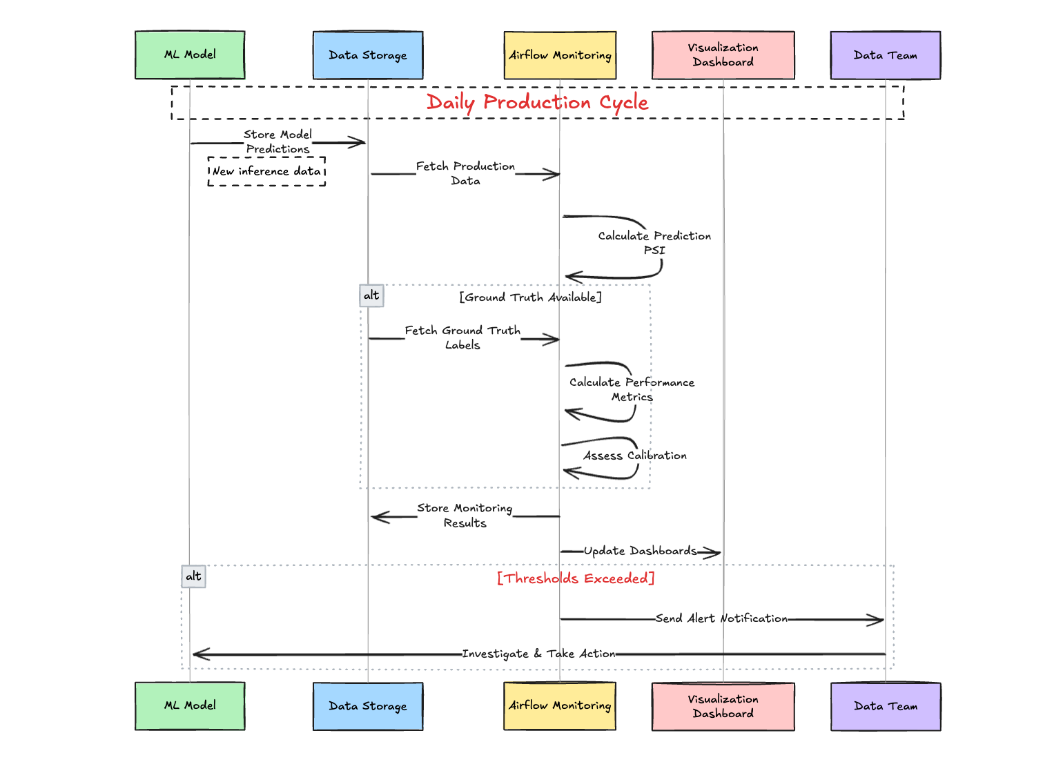
Example Model Performance Monitoring Process:
-
Daily Workflow:
- ML model stores predictions in database
- Airflow pipeline fetches production data
- System calculates Prediction PSI to detect drift
-
When Ground Truth Available:
- System retrieves actual outcomes
- Calculates performance metrics (AUC, F1)
- Assesses model calibration
-
Reporting & Response:
- Stores all monitoring results
- Updates visualization dashboards
- Sends alerts if thresholds exceeded
- Data team investigates and takes action when needed
6. Automating Monitoring with Apache Airflow
Manual monitoring is impractical for production ML systems where data flows continuously and issues can emerge at any time. Automation ensures consistency, scalability, and timely detection of problems. Apache Airflow, a powerful open-source platform, excels at orchestrating complex workflows by defining them as Directed Acyclic Graphs (DAGs). Let’s explore how to automate the monitoring tasks we’ve discussed—prediction PSI, performance metrics, and calibration—using Airflow.
Setting Up an Airflow DAG for ML Monitoring
Here’s a practical example of an Airflow DAG that runs daily monitoring checks on your ML model’s predictions and performance:
1from airflow import DAG
2from airflow.operators.python import PythonOperator
3from airflow.utils.dates import days_ago
4import pandas as pd
5import logging
6from datetime import timedelta
7import numpy as np
8from sklearn.metrics import roc_auc_score
9# Assume these are defined elsewhere (from Section 5)
10from your_module import calculate_psi, check_performance, check_calibration
11# Dummy data fetcher (replace with real data source like SQL, S3, etc.)
12def fetch_data(is_reference=False):
13    np.random.seed(42 if is_reference else None)
14    data = pd.DataFrame({
15            'score': np.clip(np.random.normal(0.5 if is_reference else 0.6, 0.1, 1000), 0.01, 0.99),
16        'label': (np.random.normal(0, 0.2, 1000) + (0.5 if is_reference else 0.6) > 0.6).astype(int)
17    })
18    return data
19def monitor_predictions(**kwargs):
20    ref_data = fetch_data(is_reference=True)  # Reference dataset (e.g., training/validation)
21    new_data = fetch_data(is_reference=False)  # New production data
22    psi_score = calculate_psi(ref_data['score'], new_data['score'])
23    logging.info(f"Prediction PSI: {psi_score:.3f}")
24    if psi_score > 0.2:
25        logging.warning(f"High PSI detected: {psi_score:.3f}")
26    kwargs['ti'].xcom_push(key='psi_score', value=psi_score)  # Pass PSI to downstream tasks
27def monitor_performance(**kwargs):
28    new_data = fetch_data(is_reference=False)
29    auc_score = check_performance(new_data['label'], new_data['score'], metric='auc')
30    logging.info(f"AUC Score: {auc_score:.3f}")
31    kwargs['ti'].xcom_push(key='auc_score', value=auc_score)
32def monitor_calibration(**kwargs):
33    new_data = fetch_data(is_reference=False)
34    cal_rmse = check_calibration(new_data['label'], new_data['score'])
35    logging.info(f"Calibration RMSE: {cal_rmse:.3f}")
36    kwargs['ti'].xcom_push(key='cal_rmse', value=cal_rmse)
37def generate_report(**kwargs):
38    ti = kwargs['ti']
39    psi_score = ti.xcom_pull(key='psi_score', task_ids='monitor_predictions')
40    auc_score = ti.xcom_pull(key='auc_score', task_ids='monitor_performance')
41    cal_rmse = ti.xcom_pull(key='cal_rmse', task_ids='monitor_calibration')
42    report = f"Monitoring Report:
43PSI: {psi_score:.3f}
44AUC: {auc_score:.3f}
45Calibration RMSE: {cal_rmse:.3f}"
46    logging.info(report)
47    # Optionally save to file, database, or send via email/Slack
48    with open('/path/to/report.txt', 'w') as f:
49        f.write(report)
50# Define the DAG
51default_args = {
52        'owner': 'ml_team',
53    'depends_on_past': False,
54    'email_on_failure': True,
55    'email': ['ml_team@example.com'],
56    'retries': 1,
57    'retry_delay': timedelta(minutes=5),
58}
59with DAG(
60        'ml_model_monitoring',
61    default_args=default_args,
62    description='Daily ML model monitoring pipeline',
63    schedule_interval=timedelta(days=1),  # Run daily
64    start_date=days_ago(1),
65    catchup=False,
66) as dag:
67    t1 = PythonOperator(
68            task_id='monitor_predictions',
69        python_callable=monitor_predictions,
70        provide_context=True,
71    )
72    t2 = PythonOperator(
73            task_id='monitor_performance',
74        python_callable=monitor_performance,
75        provide_context=True,
76    )
77    t3 = PythonOperator(
78            task_id='monitor_calibration',
79        python_callable=monitor_calibration,
80        provide_context=True,
81    )
82    t4 = PythonOperator(
83            task_id='generate_report',
84        python_callable=generate_report,
85        provide_context=True,
86    )
87    # Define task dependencies
88        [t1, t2, t3] >> t4  # All monitoring tasks must complete before report generation
89    ```
90### How It Works
911. **Tasks**: The DAG includes four tasks:
92   - `monitor_predictions`: Calculates PSI for prediction scores against a reference dataset.
93   - `monitor_performance`: Computes AUC when ground truth is available.
94   - `monitor_calibration`: Assesses calibration RMSE.
95   - `generate_report`: Aggregates results into a report, which could be saved, emailed, or sent to a Slack channel.
962. **Scheduling**: The `schedule_interval` runs the DAG daily, but you can adjust this (e.g., hourly with `timedelta(hours=1)`).
973. **Data Fetching**: The `fetch_data` function simulates data retrieval. In practice, replace it with queries to a database (e.g., PostgreSQL via `PostgresOperator`), cloud storage (e.g., S3 via `S3Hook`), or an API.
984. **XCom**: Airflow’s XCom system passes metrics between tasks, enabling the report task to compile results.
995. **Alerts**: Configure Airflow to send emails or Slack notifications on failure or when thresholds are breached (e.g., using `SlackWebhookOperator`).
100### Extending the DAG
101- **Feature Monitoring**: Add tasks from Part 1 (e.g., null checks, feature PSI) as parallel tasks feeding into the report.
102- **Storage**: Persist metrics to a database (e.g., via `PostgresOperator`) or a time-series store like Prometheus for trend analysis.
103- **Dynamic Thresholds**: Incorporate logic to adjust thresholds based on historical performance or business SLOs.
104**Why It Matters**: Automation with Airflow reduces human error, ensures timely checks, and scales with your ML system’s complexity. It integrates seamlessly with existing data pipelines and can trigger downstream actions (e.g., retraining) based on monitoring outcomes.
105---
106## 7. Visualizing Insights for Action
107Raw metrics and logs are vital, but visualizations transform them into actionable insights. By presenting drift, performance, and calibration trends graphically, you enable faster detection of issues and clearer communication with stakeholders—technical and non-technical alike. Tools like Looker, Tableau, Grafana, or even custom Python plots can bring your monitoring data to life.
108### Example Visualization Workflow
109Assume your Airflow pipeline stores monitoring results (PSI, AUC, calibration RMSE) in a database like PostgreSQL or a data warehouse like BigQuery. Here’s how to visualize them:
110#### Using Looker for Dashboards
1111. **Connect Data Source**:
112   - Link Looker to your database or warehouse where monitoring metrics are stored (e.g., a table with columns: `timestamp`, `psi_score`, `auc_score`, `cal_rmse`).
113   - Define a LookML model to structure your data (e.g., a `monitoring_metrics` view).
1142. **Key Visualizations**:
115   - **Prediction PSI Over Time**:
116     - Create a line chart with `timestamp` on the x-axis and `psi_score` on the y-axis.
117     - Add a reference line at PSI = 0.2 to highlight significant drift.
118     - Example LookML:
119```lookml
120measure: avg_psi {
121     type: average
122 sql: ${psi_score} ;;
123}
124dimension_group: monitor_time {
125     type: time
126 sql: ${timestamp} ;;
127 timeframes: [date, week, month]
128}
- Performance Metrics Trend:
- Plot
auc_scoreover time as a line chart. - Add a threshold line (e.g., AUC = 0.7) and color-code drops below it.
- Plot
- Calibration Reliability Diagram:
- Use a scatter plot with
mean_predicted_value(fromcalibration_curve) on the x-axis andfraction_of_positiveson the y-axis, overlaying the ideal y=x line. - This might require pre-computing bins in your pipeline and storing them.
- Use a scatter plot with
- Dashboard Assembly:
- Combine these visuals into a Looker dashboard.
- Add filters (e.g., date range, model version) and titles like "ML Model Health Overview."
- Schedule automatic refreshes (e.g., daily) to reflect the latest Airflow runs.
Alternative Tools
- Grafana: Ideal for time-series data. Connect it to a time-series database (e.g., Prometheus, InfluxDB) where Airflow pushes metrics. Use panels for PSI trends, AUC drops, and calibration RMSE, with alerting rules for thresholds.
- Tableau: Similar to Looker, connect to your data source and build interactive dashboards. Great for business stakeholders who prefer drag-and-drop interfaces.
- Python (Matplotlib/Seaborn): Generate plots in your Airflow
generate_reporttask and save them as images or PDFs:1import matplotlib.pyplot as plt 2import seaborn as sns 3def plot_metrics(history_df: pd.DataFrame, output_path: str): 4 plt.figure(figsize=(10, 6)) 5 sns.lineplot(data=history_df, x='date', y='psi_score', label='PSI') 6 plt.axhline(0.2, color='red', linestyle='--', label='PSI Threshold') 7 plt.title('Prediction PSI Over Time') 8 plt.legend() 9 plt.savefig(f"{output_path}/psi_trend.png") 10 plt.close()- Upload these to cloud storage (e.g., S3) or attach them to notifications.
Other Useful Visualizations
- Metrics Over Time: Track PSI, AUC, F1, or calibration RMSE across monitoring runs. A sudden spike in PSI or drop in AUC signals immediate attention.
- Feature Importance Drift: For interpretable models, plot SHAP values or feature importances over time to spot shifts in what drives predictions.
- Calibration Curves: Use reliability diagrams (as shown in Section 5) to visualize miscalibration trends, especially when RMSE exceeds your threshold.
Other Useful Visualizations:
- Metrics Over Time: Plot PSI, AUC, F1-score, null rates, calibration RMSE, etc., over consecutive monitoring runs (e.g., daily, weekly). This requires storing monitoring results persistently (e.g., in a database, metrics store like Prometheus, or even just files in cloud storage). Time series plots quickly reveal trends, seasonality, or sudden drops/spikes.
- Feature Importance Drift: If your model allows interpretation (e.g., tree-based models, linear models), track how feature importances change over time compared to the training baseline. A significant shift might indicate concept drift where different factors become more/less predictive. Libraries like SHAP can help calculate importance values consistently.
- Calibration Curves (Reliability Diagrams): Plot
fraction_of_positivesvs.mean_predicted_valuefromcalibration_curve. A perfectly calibrated model follows the y=x diagonal. Deviations highlight miscalibration. Why It Matters: Visual dashboards provide an intuitive overview of model health, allowing teams (including non-technical stakeholders) to quickly spot anomalies that might be missed in raw logs or tables. They are crucial for communication and faster decision-making.
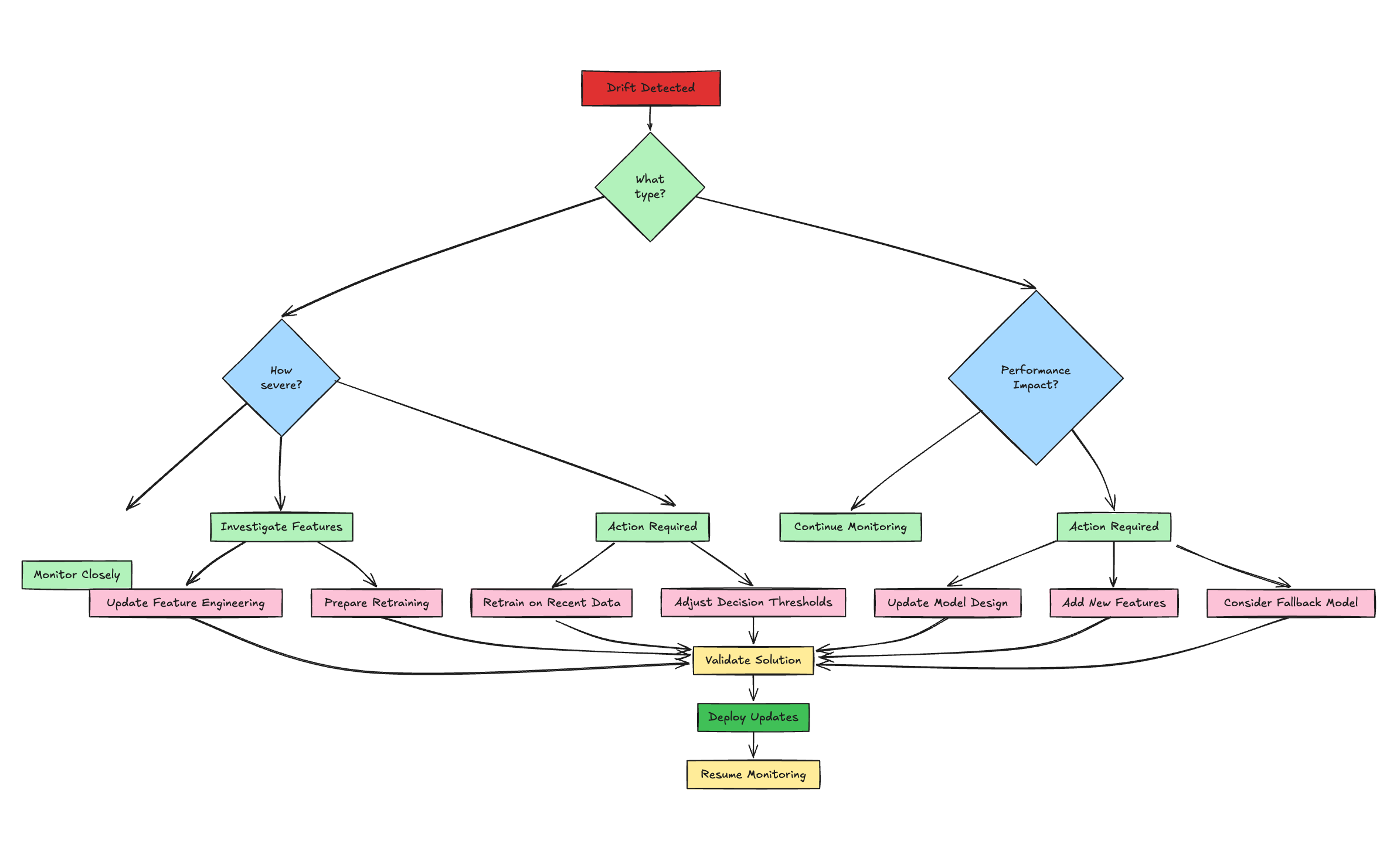
8. Responding to Drift: Strategies for Resilience
Detecting drift is just the starting point—acting on it is what keeps your ML system robust. Responses should align with the drift’s type, severity, and business impact. Below are structured strategies to ensure resilience.
Diagnose the Issue
- Pinpoint the Cause:
- Check upstream pipelines (logs, errors) and feature-level metrics (CSI, nulls, outliers from Part 1) to distinguish real drift from data quality issues.
- Differentiate data drift (shifting feature distributions) from concept drift (performance drop on recent labeled data or shifting feature importance).
- Assess sudden vs. gradual drift using visualization trends—sudden shifts may indicate pipeline failures, while gradual changes suggest evolving behavior.
- Why It Matters: Accurate diagnosis guides the right response, avoiding wasted effort.
Decide on Action
- Monitor Minor Drift:
- If PSI < 0.1-0.15 or performance dips are within SLOs, continue monitoring without action. Predefine acceptable thresholds with stakeholders.
- Alert & Escalate:
- Route alerts (e.g., via Airflow, Slack, PagerDuty) to the right team based on severity—moderate drift triggers investigation, severe drift demands immediate response.
- Adjust Thresholds:
- For classifiers, tweak decision thresholds to mitigate impact temporarily, balancing precision/recall trade-offs without retraining.
- Retrain or Redesign:
- Simple Retraining: Use recent data with the same model for data drift; schedule regularly or trigger on thresholds (e.g., PSI > 0.2).
- Full Redevelopment: Address concept drift with new features, models, or hyperparameters if simple retraining fails.
- Fallback Model:
- Switch to a simpler, robust baseline (e.g., logistic regression) during severe issues to maintain service while fixing the primary model.
- Fix Feature Engineering:
- Update logic (cleaning, encoding) for specific drifting features, often faster than retraining.
Close the Loop
- Feedback to Development: Use drift insights to refine feature selection, model design, and data strategies for future iterations.
- Standardize Responses: Create a playbook with clear SOPs, roles, and responsibilities for each scenario to ensure consistent, timely action. Why It Matters: A structured response turns drift detection into resilience, minimizing downtime and maintaining trust in your ML system.
9. Best Practices and Next Steps
Reliable ML in production demands proactive, embedded monitoring. Here’s a concise guide to best practices and future directions.
Core Best Practices
- Monitor Holistically: Cover inputs (data quality), outputs (drift, performance), and operations (latency, errors).
- Automate Everything: Use tools like Airflow, Kubeflow, or cloud-native pipelines to eliminate manual checks.
- Set Clear Triggers: Define thresholds (e.g., PSI > 0.2, AUC drop > 10%) tied to business impact, with actionable alerts to avoid fatigue.
- Visualize Effectively: Build dashboards (Looker, Grafana, Tableau) for trends and anomalies, accessible to all teams.
- Version Control: Track schemas, code, datasets, and models for reproducibility and debugging.
- Ensure Fairness: Monitor bias metrics (e.g., demographic parity) in high-stakes use cases, integrating into pipelines.
- Plan Responses: Document alert handling (per Section 8) with clear ownership.
- Start Simple: Begin with basic checks (nulls, PSI, AUC), then scale to advanced monitoring (calibration, fairness).
- Persist Metrics: Store results in databases or time-series stores (e.g., Prometheus) for trend analysis.
Next Steps for Growth
- Adopt Specialized Tools: Explore platforms like Evidently AI, Arize for advanced drift detection and explainability with minimal coding.
- Link to Experimentation: Integrate with MLflow or Weights & Biases to connect production metrics to training runs.
- Go Real-Time: Implement online monitoring for streaming data, enabling instant interventions like traffic shifts. Why It Matters: These practices embed monitoring into MLOps, ensuring models stay effective and fair. Start with the basics, then evolve with your system’s needs.
10. Conclusion (Series Wrap-up)
Continuous monitoring isn't an optional add-on; it's a fundamental requirement for deploying and maintaining reliable, effective, and fair machine learning models in production. Models inevitably encounter drift and performance degradation as the real world diverges from the data they were trained on. Throughout this two-part guide, we've built a framework for tackling this challenge:
- We established the critical need for monitoring and explored the various types of drift.
- In Part 1, we detailed how to safeguard model inputs through rigorous feature monitoring (checking nulls, distributions via PSI, outliers, cardinality, etc.).
- In Part 2, we shifted focus to model outputs, covering prediction drift, performance metric tracking (AUC, F1), and calibration. We then demonstrated how to automate these checks using Apache Airflow, stressed the importance of visualization, and outlined practical strategies for responding to detected issues. Finally, we summarized best practices for embedding monitoring into your MLOps workflow. By implementing a systematic, automated approach using tools like Python, stability indices, performance metrics, and workflow orchestrators, you can build trust in your models, catch issues before they cause significant harm, and ensure your ML systems continue to deliver value effectively and responsibly even as the world changes. Start implementing these practices today to safeguard your ML investments and build more resilient AI systems.
11. References
- Evidently AI: ML Monitoring
- Google Cloud: ML Model Monitoring (Platform-specific example and concepts)
- MachineLearningPlus: Population Stability Index (PSI) (Detailed PSI explanation)
- Understanding Model Calibration in Machine Learning(About Model Calibration)
- Apache Airflow Documentation