Continuous Model Monitoring in Machine Learning (Part 1): Why It's Crucial and How to Monitor Your Inputs

You've trained a stellar machine learning model, tested it rigorously, and deployed it into productions, congratulations! But how do you ensure it keeps delivering spot-on predictions as the world around it shifts?

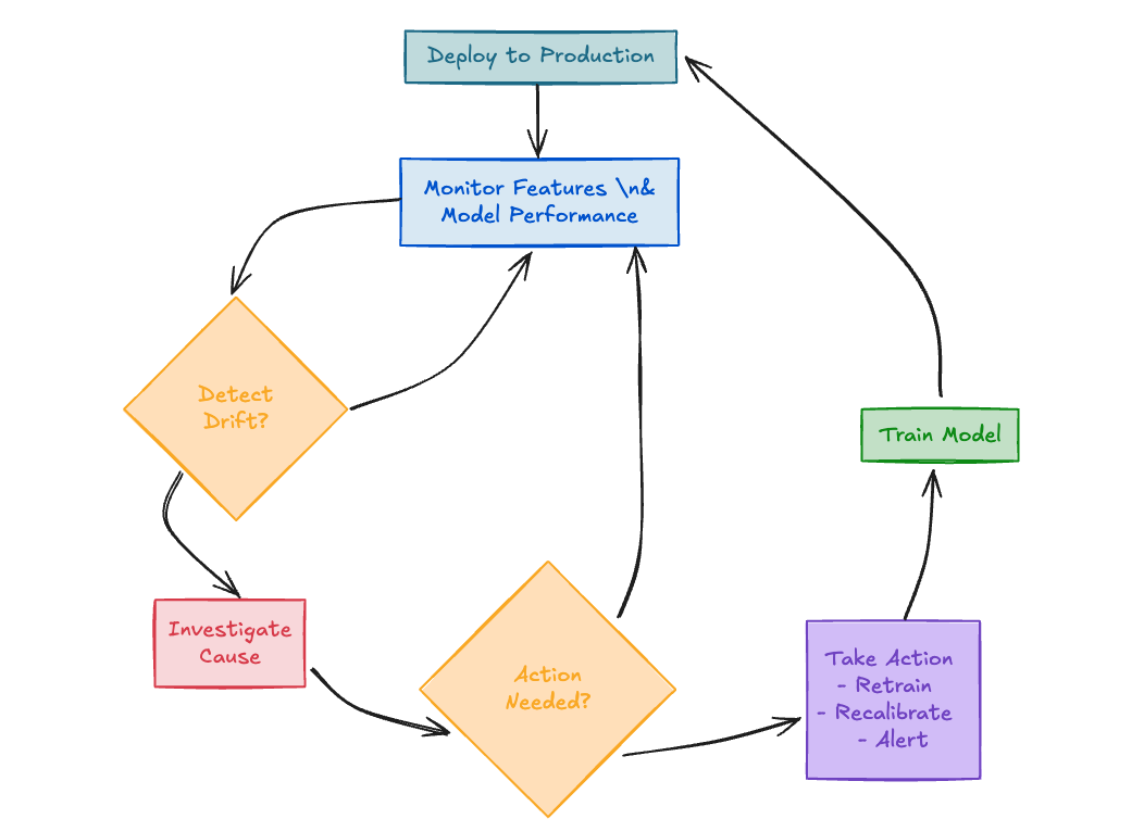
Machine learning models are built on historical data, but production environments are dynamic—user behaviors evolve, external events disrupt patterns, and data pipelines can falter. Studies suggest ML models can lose significant accuracy within months without proper monitoring. This introduces data drift, concept drift, and other issues that can silently erode your model's performance, reliability, and fairness over time. The solution? Continuous model monitoring—a proactive, systematic approach to tracking feature health, model performance, and drift, ensuring your predictions stay trustworthy and effective.

This series will guide you through building a robust monitoring framework using Python, Apache Airflow, and industry-standard techniques. In Part 1, we'll lay the groundwork, covering why monitoring is essential, understanding the types of drift you'll encounter, and diving deep into monitoring your model's input features and detecting basic distribution shifts.

Here's what we'll cover in Part 1:

1. Why Continuous Monitoring is Non-Negotiable
2. Understanding Data Drift: Types and Triggers
3. Feature Monitoring: Safeguarding Your Inputs (Nulls, Percentiles, Outliers, Consistency, Timeliness, Fairness, Cardinality, Correlation)
4. Detecting Drift with Stability Indices (PSI & CSI)

(Part 2 will cover Model Performance & Output Monitoring, Automation with Airflow, Visualization, Response Strategies, and Best Practices.)

---

1. Why Continuous Monitoring is Non-Negotiable?

Machine learning models are static by nature—trained on a snapshot of the past—but the real world doesn't sit still. Imagine a fraud detection model excelling in 2023, only to stumble in 2025 as online transaction patterns shift, or a recommendation system missing the mark as user preferences evolve. These scenarios reveal a harsh reality: models don't adapt unless you make them.

In production, data changes due to:

• External Shocks: Pandemics, economic shifts, or new technologies (like evolving payment methods) can rewrite patterns overnight.
• Natural Evolution: Features like income or age drift as populations and markets change.
• Data Pipeline Issues: Missing values, format errors, upstream data source changes, or stale inputs can creep in unnoticed.
• Regulatory Changes: New compliance requirements in finance, healthcare, and other regulated industries may affect model performance and validity (e.g., fairness constraints).

This evolution leads to phenomena like data drift (changes in input distributions) and concept drift (changes in the relationship between inputs and the target), threatening accuracy and trust. Without monitoring, these issues can fester, potentially costing revenue, damaging credibility, or leading to non-compliance in regulated domains like finance or healthcare.

Continuous monitoring turns the tide by:

• Tracking Features: Catching data quality issues like nulls or outliers early.
• Detecting Drift: Spotting shifts in data distributions or model predictions to preempt failures.
• Monitoring Performance: Ensuring predictions align with reality over time, using metrics where ground truth is available (covered in Part 2).
• Ensuring Compliance & Fairness: Maintaining regulatory requirements and ethical standards under frameworks like GDPR, FCRA, and AI fairness guidelines.

Think of it as your model's essential health check and early warning system—vital for keeping predictions sharp and stakeholders confident.

---

2. Understanding Data Drift: Types and Triggers

Drift is the root of many model woes in production, and it comes in multiple flavors. To build a robust monitoring system, you need to know what you're up against.

Concept Drift

Concept drift occurs when the underlying relationship between input features and the target variable changes. The patterns the model learned no longer hold true.

• Example: A churn model trained before widespread adoption of a new communication channel might incorrectly interpret increased usage of that channel. What once signaled dissatisfaction might now indicate engagement.
• Trigger: Often caused by external events, changing user behavior, or evolution in the underlying process being modeled.

Covariate Shift (Data Drift)

Covariate shift (or simply data drift) happens when the distribution of the input features (X) changes between the training and production environment, even if the relationship between features and the target (P(y|X)) remains the same.

• Example: A credit scoring model trained on incomes from 2022 might see performance degrade in 2025 if significant inflation alters the mean and variance of the 'income' feature in the production data.
• Trigger: Shifts in demographics, market conditions, data collection processes, or upstream data generation.

Beyond Features and Outputs

Drift isn't limited to just feature distributions or concept changes:

• Prediction Drift: The distribution of the model's output scores or predictions changes over time. This can be a symptom of covariate or concept drift. (More in Part 2)
• Data Quality Drift: Increases in null rates, outliers, or data inconsistencies can mimic or amplify other forms of drift.
• Timeliness Drift: Delays in data availability can make predictions less relevant, especially for real-time systems.
• Bias Drift: Shifts in the distributions or relationships concerning sensitive attributes (e.g., age, gender, location) can introduce or exacerbate fairness issues.
• Label Drift: Changes in how the ground truth labels are defined, collected, or interpreted over time.

Understanding these dynamics is crucial for designing a comprehensive monitoring strategy that covers data inputs, model outputs, and performance.

---

3. Feature Monitoring: Safeguarding Your Inputs

Features are the foundation of your model—when they wobble, predictions can crumble. Monitoring key aspects of your input features is the first line of defense. Let's look at monitoring null rates, percentiles, outliers, consistency, timeliness, fairness, cardinality, and correlation shifts, each with reusable Python code.

1import pandas as pd
2import numpy as np
3import logging
4from datetime import datetime, timezone
5
6# Set up basic logging
7logging.basicConfig(level=logging.INFO,
8                    format='%(asctime)s - %(levelname)s - %(message)s')
9
10# --- Placeholder DataFrames for Examples (replace with your actual data loading) ---
11np.random.seed(0)
12ref_data = pd.DataFrame({'income': np.random.lognormal(mean=np.log(50000), sigma=0.5, size=1000),
13                         'age': np.random.randint(18, 70, size=1000)})
14ref_data['region'] = np.random.choice(['North', 'South', 'East', 'West'], size=1000)
15ref_data['feature2'] = ref_data['income'] * 0.5 + np.random.normal(0, 10000, len(ref_data)) # Added for correlation example
16
17new_data_stable = pd.DataFrame({'income': np.random.lognormal(mean=np.log(51000), sigma=0.5, size=1000),
18                                'age': np.random.randint(18, 72, size=1000)}) # Slightly different age range
19new_data_stable['region'] = np.random.choice(['North', 'South', 'East', 'West'], size=1000)
20new_data_stable['feature2'] = new_data_stable['income'] * 0.51 + np.random.normal(0, 10500, len(new_data_stable))
21
22new_data_shifted = pd.DataFrame({'income': np.random.lognormal(mean=np.log(60000), sigma=0.6, size=1000),
23                                 'age': np.random.randint(25, 80, size=1000)}) # Shifted age range
24new_data_shifted['income'].iloc[::10] = np.nan # Introduce nulls
25new_data_shifted['region'] = np.random.choice(['North', 'South', 'East', 'West', 'Central'], size=1000) # New category
26new_data_shifted['feature2'] = new_data_shifted['income'] * 0.1 + np.random.normal(0, 5000, len(new_data_shifted)) # Weaker correlation
27
28data_time = pd.DataFrame({
29    'event_time': pd.to_datetime(['2025-04-05 10:00:00', '2025-04-05 23:00:00', '2025-04-06 07:00:00']),
30    'value': [1, 2, 3]
31})
32
33fair_data = pd.DataFrame({
34    'score': [0.6, 0.7, 0.65, 0.55, 0.75, 0.68],
35    'group': ['A', 'B', 'A', 'B', 'A', 'B']
36})
37# --- End Placeholder DataFrames ---

Monitoring Null Rates

Missing data can skew results or even cause pipelines to fail. Tracking the percentage of nulls is fundamental.

1def check_nulls(df: pd.DataFrame, feature: str, threshold: float = 0.1) -> float:
2    """Check null rate for a feature and log a warning if it exceeds the threshold."""
3    if feature not in df.columns:
4        logging.error(f"Feature '{feature}' not found in dataframe.")
5        return float('nan')
6
7    null_rate = df[feature].isnull().mean()
8
9    if null_rate > threshold:
10        logging.warning(f"ALERT [{feature}]: Null rate is {null_rate:.2%}, exceeding threshold {threshold:.0%}!")
11    else:
12        logging.info(f"Check [{feature}]: Null rate stable at {null_rate:.2%}.")
13
14    return null_rate
15
16# Example
17check_nulls(new_data_shifted, 'income', threshold=0.05) # Example: Logs warning for 10% nulls
18check_nulls(new_data_stable, 'income', threshold=0.05) # Example: Logs info for 0% nulls

Why It Matters: A sudden spike in nulls often indicates an upstream data pipeline failure or a change in data collection—critical to catch early.

Monitoring Percentiles (e.g., p50, p90, p99)

Percentiles help understand the shape of a feature's distribution and how it changes, especially in the tails (p90, p99), crucial for skewed features.

1def check_percentiles(df: pd.DataFrame, feature: str,
2                      percentiles: list = [0.5, 0.9, 0.99],
3                      ref_values: dict = None, tolerance: float = 0.1) -> dict:
4    """Check feature percentiles and compare to reference values with a relative tolerance."""
5    if feature not in df.columns:
6        logging.error(f"Feature '{feature}' not found in dataframe.")
7        return {}
8    if not pd.api.types.is_numeric_dtype(df[feature]):
9        logging.warning(f"Feature '{feature}' is not numeric, skipping percentile check.")
10        return {p: float('nan') for p in percentiles}
11
12    valid_data = df[feature].dropna()
13    if len(valid_data) == 0:
14        logging.error(f"No valid data for percentile calculation in feature '{feature}'.")
15        return {p: float('nan') for p in percentiles}
16
17    p_values = valid_data.quantile(percentiles).to_dict()
18
19    if ref_values:
20        alerts = []
21        for p in percentiles:
22            if p in ref_values and p in p_values and not np.isnan(ref_values[p]) and not np.isnan(p_values[p]):
23                ref_val = ref_values[p]
24                curr_val = p_values[p]
25                if abs(ref_val) > 1e-6:
26                    rel_diff = abs(curr_val - ref_val) / abs(ref_val)
27                    if rel_diff > tolerance:
28                        alerts.append(f"p{int(p*100)} changed by {rel_diff:.1%} (from {ref_val:.2f} to {curr_val:.2f})")
29                elif abs(curr_val - ref_val) > 1e-6: # Handle case where ref is zero but current is not
30                    alerts.append(f"p{int(p*100)} changed significantly from zero to {curr_val:.2f}")
31
32        if alerts:
33            logging.warning(f"ALERT [{feature}]: Percentile shifts detected: {', '.join(alerts)} (tolerance {tolerance:.0%}).")
34        else:
35            logging.info(f"Check [{feature}]: Percentiles stable within tolerance.")
36    else:
37        logging.info(f"Check [{feature}]: Calculated percentiles: {p_values}")
38
39    return p_values
40
41# Example
42ref_p = check_percentiles(ref_data, 'income') # Calculate baseline
43check_percentiles(new_data_stable, 'income', ref_values=ref_p, tolerance=0.1) # Should be stable
44check_percentiles(new_data_shifted, 'income', ref_values=ref_p, tolerance=0.1) # Should trigger alert

Why It Matters: A jump in p99 might indicate an increase in extreme values (potential outliers or fraud), while a shift in p50 (median) signals a change in the central tendency.

Monitoring Outliers

Extreme values can disproportionately influence some models or indicate data errors.

1def check_outliers(df: pd.DataFrame, feature: str, method: str = 'iqr',
2                   threshold: float = 0.05,
3                   params: dict = {'iqr_multiplier': 1.5, 'std_multiplier': 3}) -> float:
4    """Detect the rate of outliers using IQR or Z-score method and log alert if threshold exceeded."""
5    if feature not in df.columns:
6        logging.error(f"Feature '{feature}' not found in dataframe.")
7        return float('nan')
8    if not pd.api.types.is_numeric_dtype(df[feature]):
9        logging.warning(f"Feature '{feature}' is not numeric, skipping outlier detection.")
10        return 0.0 # Return 0 rate for non-numeric
11
12    values = df[feature].dropna()
13    if len(values) < 10: # Need sufficient data points
14        logging.info(f"Check [{feature}]: Insufficient data ({len(values)} points) for robust outlier detection.")
15        return 0.0
16
17    outliers_idx = pd.Series(False, index=df.index) # Default to no outliers
18
19    try:
20        if method == 'iqr':
21            q1, q3 = values.quantile([0.25, 0.75])
22            iqr = q3 - q1
23            lower_bound = q1 - params.get('iqr_multiplier', 1.5) * iqr
24            upper_bound = q3 + params.get('iqr_multiplier', 1.5) * iqr
25            # Apply outlier logic to the original dataframe's index where the feature is not NaN
26            outliers_idx.loc[values[(values < lower_bound) | (values > upper_bound)].index] = True
27        elif method == 'zscore':
28            mean, std = values.mean(), values.std()
29            if std > 1e-6: # Avoid division by zero/instability
30                z_scores = (values - mean) / std
31                mult = params.get('std_multiplier', 3)
32                # Apply z-score logic to the original dataframe index
33                outliers_idx.loc[values[abs(z_scores) > mult].index] = True
34            else:
35                logging.warning(f"Check [{feature}]: Standard deviation is near zero, cannot use Z-score method.")
36                return 0.0
37        else:
38            logging.error(f"Unknown outlier detection method: {method}")
39            return float('nan')
40
41        # Calculate rate based on the original dataframe size (including potential NaNs)
42        rate = outliers_idx.sum() / len(df)
43
44        if rate > threshold:
45            logging.warning(f"ALERT [{feature}]: Outlier rate is {rate:.2%}, exceeding threshold {threshold:.0%}!")
46        else:
47            logging.info(f"Check [{feature}]: Outlier rate stable at {rate:.2%}.")
48
49        return rate
50    except Exception as e:
51        logging.error(f"Error during outlier detection for {feature}: {e}")
52        return float('nan')
53
54# Example using the shifted data which might have more outliers
55check_outliers(new_data_shifted, 'income', threshold=0.05)
56check_outliers(new_data_stable, 'income', threshold=0.05)

Why It Matters: Outliers might represent data entry errors, sensor malfunctions, or genuine but rare events. Identifying changes in their frequency is crucial.

Monitoring Consistency (Example: Between Two Sources)

If a feature comes from multiple pipelines or sources, ensure its characteristics (like the mean) are consistent. (This example compares means, adapt as needed)

1def check_consistency(df1: pd.DataFrame, df2: pd.DataFrame, feature: str, tolerance: float = 0.05) -> float:
2    """Check if the mean of a feature is consistent across two dataframes within a relative tolerance."""
3    if feature not in df1.columns or feature not in df2.columns:
4        logging.error(f"Feature '{feature}' not found in both dataframes.")
5        return float('nan')
6    if not pd.api.types.is_numeric_dtype(df1[feature]) or not pd.api.types.is_numeric_dtype(df2[feature]):
7        logging.warning(f"Feature '{feature}' is not numeric in both dataframes, skipping consistency check.")
8        return float('nan')
9
10    mean1 = df1[feature].mean()
11    mean2 = df2[feature].mean()
12
13    if abs(mean1) < 1e-6: # Handle base mean near zero
14        if abs(mean2) > 1e-6:
15            rel_diff = float('inf') # Consider any non-zero diff large
16        else:
17            rel_diff = 0.0
18    else:
19        rel_diff = abs(mean1 - mean2) / abs(mean1)
20
21    if rel_diff > tolerance:
22        logging.warning(f"ALERT [{feature}]: Mean inconsistent between sources. Mean1={mean1:.2f}, Mean2={mean2:.2f} (Relative Diff: {rel_diff:.2%}, Tolerance: {tolerance:.0%})")
23    else:
24        logging.info(f"Check [{feature}]: Mean consistent between sources (Relative Diff: {rel_diff:.2%}).")
25
26    return rel_diff
27
28# Example
29check_consistency(ref_data, new_data_stable, 'income', tolerance=0.1) # Likely consistent
30check_consistency(ref_data, new_data_shifted, 'income', tolerance=0.1) # Likely inconsistent

Why It Matters: Inconsistent data between sources points to potential pipeline misalignments, processing errors, or definition mismatches.

Monitoring Timeliness

For models relying on fresh data, monitoring data latency is vital.

1def check_timeliness(df: pd.DataFrame, timestamp_col: str, max_lag_hours: float = 24.0) -> float:
2    """Check the maximum data lag compared to the current time."""
3    if timestamp_col not in df.columns:
4        logging.error(f"Timestamp column '{timestamp_col}' not found.")
5        return float('nan')
6
7    try:
8        timestamps = pd.to_datetime(df[timestamp_col], errors='coerce').dropna()
9        if timestamps.empty:
10            logging.error(f"No valid timestamps found in column '{timestamp_col}'.")
11            return float('nan')
12
13        latest_timestamp = timestamps.max()
14        # Ensure latest_timestamp is timezone-aware (assume UTC if naive)
15        if latest_timestamp.tzinfo is None:
16             latest_timestamp = latest_timestamp.tz_localize(timezone.utc)
17
18        # Ensure current time is timezone-aware (UTC)
19        now_utc = datetime.now(timezone.utc)
20
21        lag_seconds = (now_utc - latest_timestamp).total_seconds()
22        lag_hours = lag_seconds / 3600
23
24        if lag_hours < 0:
25             logging.warning(f"Check [{timestamp_col}]: Latest timestamp ({latest_timestamp}) is in the future? Lag calculated as {lag_hours:.1f} hours.")
26             # Reset lag to 0 if timestamp is in the future, could be clock skew or bad data
27             lag_hours = 0.0
28
29        if lag_hours > max_lag_hours:
30            logging.warning(f"ALERT [{timestamp_col}]: Data is stale! Maximum lag is {lag_hours:.1f} hours, exceeding threshold {max_lag_hours:.1f}h.")
31        else:
32            logging.info(f"Check [{timestamp_col}]: Data fresh. Maximum lag is {lag_hours:.1f} hours.")
33
34        return lag_hours
35    except Exception as e:
36        logging.error(f"Error checking timeliness for column '{timestamp_col}': {e}")
37        return float('nan')
38
39# Example (assuming current date is around 2025-04-06)
40check_timeliness(data_time, 'event_time', max_lag_hours=4) # Will show small lag

Why It Matters: Stale data can lead to inaccurate or irrelevant predictions, undermining the model's purpose, especially in time-sensitive applications.

Monitoring Fairness (Example: Group Disparity)

Monitor key metrics across different groups defined by sensitive attributes to detect potential bias. (This is a simple mean disparity check; adapt with more sophisticated fairness metrics as needed).

1def check_group_disparity(df: pd.DataFrame, feature: str, group_col: str, threshold: float = 0.2) -> float:
2    """Check for disparity in the mean of 'feature' across groups defined by 'group_col'."""
3    if feature not in df.columns or group_col not in df.columns:
4        logging.error(f"Feature '{feature}' or group column '{group_col}' not found.")
5        return float('nan')
6    if not pd.api.types.is_numeric_dtype(df[feature]):
7        logging.warning(f"Feature '{feature}' is not numeric, skipping group disparity check.")
8        return float('nan')
9
10    if df[group_col].nunique() < 2:
11        logging.info(f"Check [{feature}/{group_col}]: Not enough distinct groups ({df[group_col].nunique()}) for disparity check.")
12        return 0.0 # No disparity if only one group
13
14    group_means = df.groupby(group_col)[feature].mean()
15    overall_mean = df[feature].mean()
16
17    group_counts = df.groupby(group_col)[feature].count()
18    if group_counts.min() < 10:
19        logging.warning(f"Check [{feature}/{group_col}]: Some groups have very few samples (<10), mean comparison might be unstable.")
20
21    # Calculate max relative difference from overall mean
22    if abs(overall_mean) > 1e-6:
23        rel_diffs = abs(group_means - overall_mean) / abs(overall_mean)
24        max_rel_diff = rel_diffs.max()
25    elif group_means.max() > 1e-6 or group_means.min() < -1e-6: # If overall mean is zero, check if group means deviate
26        max_rel_diff = float('inf')
27    else: # All means are zero
28        max_rel_diff = 0.0
29
30    if max_rel_diff > threshold:
31        logging.warning(f"ALERT [{feature}/{group_col}]: High disparity detected. Max relative mean difference from overall: {max_rel_diff:.2%}. Threshold: {threshold:.0%}.")
32        logging.info(f"Group Means for {feature}: \n{group_means.to_string()}")
33    else:
34        logging.info(f"Check [{feature}/{group_col}]: Group means appear relatively consistent (Max Rel Diff: {max_rel_diff:.2%}).")
35
36    return max_rel_diff
37
38# Example
39check_group_disparity(fair_data, 'score', 'group', threshold=0.2) # Likely low disparity

Why It Matters: Fairness ensures ethical AI deployment and compliance. Monitoring helps catch unintended biases that might emerge due to data shifts affecting different groups differently.

Monitoring Cardinality

For categorical features, track the number of unique values.

1def check_cardinality(df: pd.DataFrame, feature: str, ref_cardinality: int = None, tolerance: float = 0.2) -> int:
2    """Check the cardinality of a categorical feature and log alerts if it shifts significantly."""
3    if feature not in df.columns:
4        logging.error(f"Feature '{feature}' not found in dataframe.")
5        return -1
6
7    current_cardinality = df[feature].nunique(dropna=True)
8
9    if ref_cardinality is None:
10        logging.info(f"Check [{feature}]: Cardinality recorded as {current_cardinality} (no reference provided).")
11    else:
12        if ref_cardinality == 0: # Handle zero reference cardinality
13             rel_change = float('inf') if current_cardinality > 0 else 0.0
14        else:
15             rel_change = abs(current_cardinality - ref_cardinality) / ref_cardinality
16
17        if rel_change > tolerance:
18            logging.warning(f"ALERT [{feature}]: Cardinality shifted significantly! Current: {current_cardinality}, Reference: {ref_cardinality} (Change: {rel_change:.2%}, Tolerance: {tolerance:.0%})")
19        else:
20            logging.info(f"Check [{feature}]: Cardinality stable at {current_cardinality} (Reference: {ref_cardinality}).")
21
22    return current_cardinality
23
24# Example
25ref_card = check_cardinality(ref_data, 'region') # Records 4
26check_cardinality(new_data_shifted, 'region', ref_cardinality=ref_card, tolerance=0.1) # Alerts for new category 'Central'

Why It Matters: A sudden change in cardinality might indicate new user behaviors, data pipeline errors, or data truncation issues.

Monitoring Correlation Shifts

Changes in correlations between features can indicate concept drift or data quality issues.

1def check_correlation_shift(ref_df: pd.DataFrame, new_df: pd.DataFrame, feature1: str, feature2: str, threshold: float = 0.2) -> float:
2    """Check for shifts in correlation between two features."""
3    if feature1 not in ref_df.columns or feature2 not in ref_df.columns or \
4       feature1 not in new_df.columns or feature2 not in new_df.columns:
5        logging.error(f"One or both features ('{feature1}', '{feature2}') not found in dataframes.")
6        return float('nan')
7
8    # Ensure features are numeric for correlation calculation
9    if not pd.api.types.is_numeric_dtype(ref_df[feature1]) or \
10       not pd.api.types.is_numeric_dtype(ref_df[feature2]) or \
11       not pd.api.types.is_numeric_dtype(new_df[feature1]) or \
12       not pd.api.types.is_numeric_dtype(new_df[feature2]):
13       logging.warning(f"One or both features ('{feature1}', '{feature2}') are not numeric. Skipping correlation check.")
14       return float('nan')
15
16    try:
17        ref_corr = ref_df[[feature1, feature2]].corr().iloc[0, 1]
18        new_corr = new_df[[feature1, feature2]].corr().iloc[0, 1]
19
20        # Handle NaN correlations (e.g., if one column becomes constant)
21        if pd.isna(ref_corr) or pd.isna(new_corr):
22            if pd.isna(ref_corr) and pd.isna(new_corr):
23                corr_diff = 0.0 # Both NaN, arguably no change
24            else:
25                corr_diff = float('inf') # One is NaN, other is not - significant change
26            logging.warning(f"Check [{feature1}-{feature2}]: Correlation calculation resulted in NaN (Ref: {ref_corr:.3f}, New: {new_corr:.3f}). Treating difference as {corr_diff}.")
27        else:
28            corr_diff = abs(new_corr - ref_corr)
29
30        if corr_diff > threshold:
31            logging.warning(f"ALERT [{feature1}-{feature2}]: Correlation shifted! Reference: {ref_corr:.3f}, Current: {new_corr:.3f} (Diff: {corr_diff:.3f}, Threshold: {threshold:.2f})")
32        else:
33            logging.info(f"Check [{feature1}-{feature2}]: Correlation stable. Reference: {ref_corr:.3f}, Current: {new_corr:.3f}")
34
35        return corr_diff
36    except Exception as e:
37        logging.error(f"Error calculating correlation shift for '{feature1}' and '{feature2}': {e}")
38        return float('nan')
39
40
41# Example
42check_correlation_shift(ref_data, new_data_stable, 'income', 'feature2', threshold=0.2) # Should be stable
43check_correlation_shift(ref_data, new_data_shifted, 'income', 'feature2', threshold=0.2) # Should show shift

Why It Matters: A shift in correlation might indicate that relationships the model relies on have changed, potentially affecting predictive power.

---

4. Detecting Drift with Stability Indices (PSI & CSI)

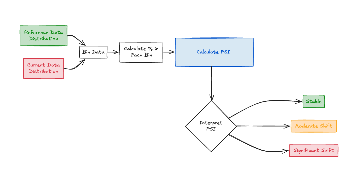
While individual feature checks are useful, we need metrics to quantify overall distribution shifts. The Population Stability Index (PSI) is an industry standard for this. Characteristic Stability Index (CSI) is simply the PSI calculated for each individual feature.

Population Stability Index (PSI)

PSI measures how much a variable's distribution has changed between two samples (e.g., training data vs. current production data). It's calculated by binning the variable and comparing the percentage of observations in each bin across the two samples.

Formula:

PSI = Σ ((Actual % in binᵢ - Expected % in binᵢ) * ln(Actual % in binᵢ / Expected % in binᵢ))

Where:

• Expected % comes from the reference dataset (e.g., training).
• Actual % comes from the current dataset being monitored.
• ln is the natural logarithm.
• Σ denotes summation across all bins i.

Interpretation Rules of Thumb:

• PSI < 0.1: No significant shift. The distribution is stable.
• 0.1 <= PSI < 0.2: Moderate shift. Monitor closely; requires attention.
• PSI >= 0.2: Significant shift. Investigation and potential action (e.g., retraining) are likely needed. (Note: Some practitioners use 0.25 as the threshold for major shift)

1def calculate_psi(ref_data: pd.Series, new_data: pd.Series, bins: int = 10) -> float:
2    """Calculates the Population Stability Index (PSI) between two distributions."""
3
4    ref_values = ref_data.dropna()
5    new_values = new_data.dropna()
6
7    if len(ref_values) == 0 or len(new_values) == 0:
8        logging.error("Cannot calculate PSI: one or both datasets have no valid data after dropping NaNs.")
9        return float('nan')
10    if not pd.api.types.is_numeric_dtype(ref_values) or not pd.api.types.is_numeric_dtype(new_values):
11        logging.warning(f"PSI calculation skipped for non-numeric feature '{ref_data.name}'.")
12        return 0.0 # Return 0 for non-numeric/categorical features where PSI isn't directly applicable this way
13
14    # Determine bin edges based on the reference data
15    min_val = ref_values.min()
16    max_val = ref_values.max()
17
18    # Handle case where min and max are the same (constant feature)
19    if min_val == max_val:
20        # If new data also has only this value, PSI is 0. If new data has different values, PSI is arguably infinite.
21        # Or if new data is empty, maybe 0 or NaN depending on convention. Let's return 0 if stable.
22        if new_values.nunique() <= 1 and (new_values.empty or new_values.iloc[0] == min_val):
23            logging.info(f"Feature '{ref_data.name}' is constant in both datasets. PSI = 0.0")
24            return 0.0
25        else:
26            logging.warning(f"Feature '{ref_data.name}' was constant in reference but changed/has NaNs in new data. Returning large PSI.")
27            return float('inf') # Indicate maximum instability
28
29
30    buffer = (max_val - min_val) * 0.001 if (max_val - min_val) > 0 else 0.01
31    # Ensure bins cover the range of both datasets if the new data exceeds the reference range
32    combined_min = min(min_val, new_values.min())
33    combined_max = max(max_val, new_values.max())
34    bin_edges = np.linspace(combined_min - buffer, combined_max + buffer, bins + 1)
35
36
37    ref_hist, _ = np.histogram(ref_values, bins=bin_edges)
38    new_hist, _ = np.histogram(new_values, bins=bin_edges)
39
40    # If total counts are zero, PSI is undefined or 0
41    if ref_hist.sum() == 0 and new_hist.sum() == 0:
42        return 0.0
43    if ref_hist.sum() == 0 or new_hist.sum() == 0:
44        # If one is empty and the other isn't, maximum drift
45        return float('inf')
46
47    eps = 1e-10 # Small epsilon to avoid division by zero or log(0)
48    ref_prop = (ref_hist + eps) / (ref_hist.sum() + eps * bins)
49    new_prop = (new_hist + eps) / (new_hist.sum() + eps * bins)
50
51    psi_components = (new_prop - ref_prop) * np.log(new_prop / ref_prop)
52    psi_value = np.sum(psi_components)
53
54    # Handle potential negative PSI due to epsilon (should be very small)
55    if psi_value < 0 and psi_value > -1e-5:
56        return 0.0
57    elif psi_value < 0:
58        logging.warning(f"Calculated negative PSI ({psi_value:.5f}) for '{ref_data.name}', possibly due to numerical issues. Clamping to 0 or check data.")
59        # Decide whether to clamp or return NaN/error, depends on tolerance for numerical issues
60        return 0.0 # Clamp small negatives to zero
61
62    return psi_value
63
64def check_distribution_drift(ref_data: pd.DataFrame, new_data: pd.DataFrame, feature: str,
65                             bins: int = 10, psi_threshold_major: float = 0.2,
66                             psi_threshold_moderate: float = 0.1) -> float:
67    """Calculates PSI for a feature and logs alerts based on thresholds."""
68    if feature not in ref_data.columns or feature not in new_data.columns:
69        logging.error(f"Feature '{feature}' not found in both dataframes for PSI calculation.")
70        return float('nan')
71
72    psi = calculate_psi(ref_data[feature], new_data[feature], bins=bins)
73
74    if np.isnan(psi):
75        logging.error(f"PSI calculation failed for feature '{feature}'.")
76    elif psi == float('inf'):
77         logging.warning(f"ALERT [{feature}]: Infinite PSI detected! Indicates major distribution divergence (e.g., constant to variable).")
78    elif psi >= psi_threshold_major:
79        logging.warning(f"ALERT [{feature}]: Significant distribution drift detected! PSI = {psi:.4f} (Threshold: {psi_threshold_major:.2f})")
80    elif psi >= psi_threshold_moderate:
81        logging.warning(f"WARNING [{feature}]: Moderate distribution drift detected. PSI = {psi:.4f} (Threshold: {psi_threshold_moderate:.2f})")
82    else:
83        logging.info(f"Check [{feature}]: Distribution stable. PSI = {psi:.4f}")
84
85    return psi
86
87# Example using previous income data
88psi_stable = check_distribution_drift(ref_data, new_data_stable, 'income') # Should be low PSI
89psi_shifted = check_distribution_drift(ref_data, new_data_shifted, 'income') # Should be high PSI
90psi_age_shifted = check_distribution_drift(ref_data, new_data_shifted, 'age') # Check age drift too
91psi_region = check_distribution_drift(ref_data, new_data_shifted, 'region') # Check non-numeric (should return 0.0 and log warning)

Why It Matters: PSI provides a single, quantitative metric to flag when a feature's distribution has changed significantly, prompting further investigation. Calculating it for each feature (CSI) helps pinpoint which inputs are driving the drift.

---

End of Part 1

In this first part, we've established why continuous monitoring is critical for maintaining reliable ML models. We explored the different types of drift that can occur and dove into practical Python code for monitoring various aspects of your input features – from basic data quality checks like nulls and outliers to detecting distribution shifts using the Population Stability Index (PSI).

Stay tuned for Part 2, where we will build upon this foundation to cover:

• Model Performance & Output Monitoring: Tracking metrics like AUC, F1-score, prediction distribution drift (PSI on scores), and calibration.
• Automating Monitoring with Apache Airflow: Setting up automated monitoring pipelines.
• Visualizing Insights: Creating plots and dashboards for effective communication.
• Responding to Drift: Strategies for investigation and remediation.
• Best Practices and Next Steps: Summarizing key takeaways and pointing towards advanced techniques.

References

• Evidently AI ML in Production Model Monitoring
• Neptune AI How to Monitor Your Models in Production Guide
• Christopher GS How to Monitor Machine Learning Models
• MachineLearningPlus Population Stability Index PSI
• Analytics Vidhya Calibration of Machine Learning Models